Recently, the researchers at Zalando, an e-commerce company, introduced Fashion MNIST as a drop-in replacement for the original MNIST dataset. Like MNIST, Fashion MNIST consists of a training set consisting of 60,000 examples belonging to 10 different classes and a test set of 10,000 examples. Each training example is a gray-scale image, 28x28 in size. The authors of the work further claim that the Fashion MNIST should actually replace MNIST dataset for benchmarking of new Machine Learning or Computer Vision models.

The rest of the post is organized as follows: We will first look at the differences between Fashion MNIST and MNIST, including performances of the model on each of the datasets. Then we will evaluate the following two claims made by the authors:

• MNIST is too easy, overused and does not adequately represent the modern Computer Vision tasks and therefore needs to be replaced.
• Fashion MNIST can act as a good drop in replacement for MNIST, since it does not have the above deficiencies.

What is MNIST Dataset?

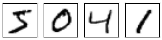
MNIST dataset is a large dataset consisting of handwriting digits which is commonly used for training and benchmarking various Machine Learning and Computer Vision models. It consists of a dataset of about 60,000 training examples. Each training example is a grayscale image of a handwritten digit on 28x28 pixels. Each training examle has a label, indicating the digit the image corresponds to. Thus, there are 10 labels (0-9) in all. This dataset was intended to be used for benchmarking various machine learning classification algorithms. However, it’s very easy for classification algorithms to achieve near-human performance on this dataset. For example, a simple k-Nearest Neighbour algorithm can achieve an accuracy of 99%. With CNNs, the performance is even better, touching 99.8%.

Since it is easy to get good accuracy for classification tasks on MNIST dataset, it is often used as a “Hello World” of Machine Learning and Computer Vision. A lot of tutorials on introduction to Machine Learning often use this dataset as example. TensorFlow, for example, has a tutorial for building classification models for MNIST dataset using its framework. Kaggle had previously hosted a “Playground” competition on the same dataset.

To get a better idea about the images, here are few examples:

Enter Fashion MNIST

While releasing this dataset, researchers at Zalando made the following observations on MNIST (Source):

• MNIST is too easy. Convolutional nets can achieve 99.7% on MNIST. Classic machine learning algorithms can also achieve 97% easily. Check out our side-by-side benchmark for Fashion-MNIST vs. MNIST, and read “Most pairs of MNIST digits can be distinguished pretty well by just one pixel.”
• MNIST is overused. In this April 2017 Twitter thread, Google Brain research scientist and deep learning expert Ian Goodfellow calls for people to move away from MNIST.
• MNIST can not represent modern CV tasks, as noted in this April 2017 Twitter thread, deep learning expert/Keras author François Chollet.

The researchers introduced Fashion-MNIST as a drop in replacement for MNIST dataset. The new dataset contains images of various clothing items - such as shirts, shoes, coats and other fashion items.

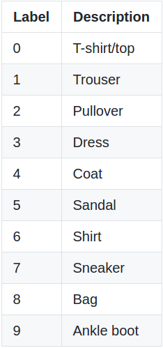
Fashion MNIST shares the shame train-test split structure as MNIST. Whereas in the case of MNIST dataset, the class labels were digits 0-9. The class labels for Fashion MNIST are:

Training a Classifier on Fashion MNIST

Let’s now move to the fun part: We will create a simple CNN based classification model to evaluate performances on MNIST dataset and its proposed replacement - Fashion MNIST. We will be building our model using the Keras framework. For more information on the framework, refer to the documentation here.

Fetching the Dataset:

The data can be obtained directly from the download links here. Alternatively, if you have access to a terminal, you can download the datasets by executing the following commands:

wget -P data/fashion http://fashion-mnist.s3-website.eu-central-1.amazonaws.com/train-images-idx3-ubyte.gz
wget -P data/fashion http://fashion-mnist.s3-website.eu-central-1.amazonaws.com/train-labels-idx1-ubyte.gz
wget -P data/fashion http://fashion-mnist.s3-website.eu-central-1.amazonaws.com/t10k-images-idx3-ubyte.gz
wget -P data/fashion http://fashion-mnist.s3-website.eu-central-1.amazonaws.com/t10k-labels-idx1-ubyte.gz

Once the datasets have been downloaded, we need to load them into the our Python session. To do this, we will be using mnist_reader provided by the authors of the dataset. The script requires NumPy.

import keras
from keras.layers import Conv2D, MaxPool2D, Flatten
from keras.layers import Dense, Dropout

import mnist_reader

X_train, y_train = mnist_reader.load_mnist('data/fashion', kind='train')
X_test, y_test = mnist_reader.load_mnist('data/fashion', kind='t10k')

Please note that the above code assumes that the dataset has beein saved in data/fashion directory. If your destination for downloads was something else, you can change it accordingly in the last two lines above.

Building a Classification Model

Now we start building our CNN based model. The model has the same architecture as the one in Tensorflow’s Tutorial on “Deep MNIST for Experts”. It consists of 2 convolution layers, each followed by a max pooling layer. The output of the second max-pooling layer is flattened and fed into a fully connected hidden layer with 1024 neurons ReLU activation function. Finally, the output layer contains 10 neurons, with softmax activation function.

model = keras.models.Sequential([
    keras.layers.Conv2D(32, (5, 5), padding="same", input_shape=[28, 28, 1]),
    keras.layers.MaxPool2D((2,2)),
    keras.layers.Conv2D(64, (5, 5), padding="same"),
    keras.layers.MaxPool2D((2,2)),
    keras.layers.Flatten(),
    keras.layers.Dense(1024, activation='relu'),
    keras.layers.Dropout(0.5),
    keras.layers.Dense(10, activation='softmax')
])

We can have a better look at the model my using model.summary(). This will generate a model summary which will look like this:

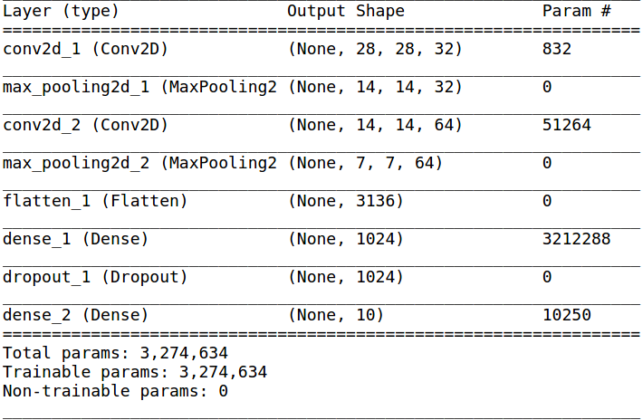
Output Shapes

Notice the column “Output Shape”. Each row in that column represents a tuple, with first element set to None. This first dimension of the output shape represents the size of the batch. Since the model is unsure of the batch size at the moment, it does not want to make any assumptions. In fact, having None as the first argument allows us to feed batches of any number of training examples, as long as the rest of the dimensions match.

For exaple, let us imagine that we had 32 examples in our first batch of inputs fed to the model. Now, each input example is a 28x28 image set, each having 1 channel (grayscale, it would have been 3 in the case of color, 1 each for Red, Green and Blue). That’s why the input_shape argument to the first Conv2D layer is (28, 28, 1), corresponding to height, width and number of channels respectively. Why don’t we need to specify input shape to other layers? Since the model is sequential, the output shape of one layer will be the input shape of the next layer.

Now, the first convolution layer gives 32 channels as output (the first argument, which reads 32), after convolving the image with 5x5 filters (second argument). The padding is “same”, which means the layer is sufficiently zero padded so that each of the 32 channel outputs have exact same height and width as the input. Therefore, the first output reads (None, 28, 28, 32), with the second, third and the fourth dimension representing height, width and number of channels respectively.

We now move to the maxpool layer. The shape of max-pooling layer is 2x2 (the first argument). We haven’t specified any stride size, and it therefore defaults to the size of the input. This means that we will make a jump of size 2 each along the height and the width dimension. For each 2x2 block the maxpool layer jumps to, it generates 1 output which is the maximum of the 4 cells of the block it spans across. This way, we are able to achieve a reduction in the size of the image. Due to this, the output of the maxpool layer consists of 32 channels, each channel being a 14x14 matrix of max-pooled data. Therefore, the output shape is (None, 14, 14, 32).

After another set of similar convolution and max-pooling layers, the input has now been transformed into a tensor with shape (batch size, 7, 7, 64). The further layers of our network are fully connected layers. These layers require the input to be a vector, whereas our data is a 3d cube of size 7x7x64. Therefore, we apply a Flatten layer. This takes the transformed data, which is in the form of a cube, and rearranges them into a flat vector having just one dimension. The number of elements in this 1d vector would be 7x7x64 = 3136.

The final 2 layers are dense layers, the output of shape of each is the same as the number of neurons in each dense layers (provided as the first argument).

Reshaping

Before we move to training, there’s one small task that needs to be done. Notice that the first layer expects the input to be of the shape (None, 28, 28, 1), whereas, if you look at the shape of the training dataset:

X_train.shape
(60000, 784)

60,000 corresponds to the number of training examples. Why 784? Because the data that we had fetched, has flattened each of the 28x28 images into single dimension of size 784. This is because most of the Machine Learning classifiers (except convolution based) expect each training example to be a vector. So, for our model, we need to reshape this 784 dimensional into images of size 28x28x1. The “1” at the end corresponds to the number of channels.

X_train = X_train.reshape([-1, 28, 28, 1])
X_test = X_test.reshape([-1, 28, 28, 1])
X_train = X_train/255
X_test = X_test/255

Most of the machine learning models work the best when the input features have been normalized, ie, they are transformed into a space of [0, 1] or [-1, 1]. In our dataset, each element for each image represents the intensity of the corresponding pixel, with a value between [0, 255]. We rescale this image by dividing each pixel’s value by 255. This scales our features to [0, 1]

The final layer of our model has 10 neurons. That means the output of our model will be a 1d vector of size 10, with each element representing a “probability score”. This score corresponds to the model’s confidence in assigning the particular class to the input example. Remember, our input belongs to one of the 10 classes enumerated in the table above. However, if we look at y_train, each label is not a 1-d vector of size 10, but a value corresponding to the correct class. We therefore need to convert the current representation of the labels to “One Hot Representation”.

y_train = keras.utils.np_utils.to_categorical(y_train)
y_test = keras.utils.np_utils.to_categorical(y_train)

Compiling and Training

We first need to compile our model before we can start training. This is because

model.compile(keras.optimizers.Adam(1e-4), loss='categorical_crossentropy', metrics=['accuracy'])
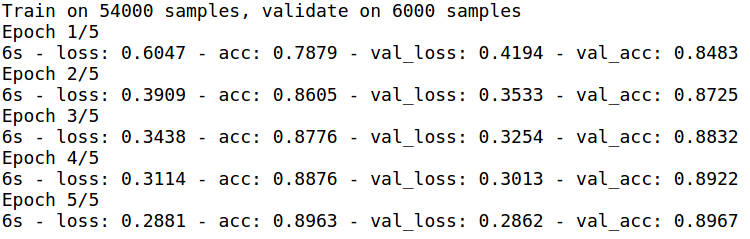
model.fit(x_train, y_train, validation_split=0.10, batch_size=64, epochs=25, verbose=2)

I have shown the output of only first 5 epochs. After 25 epochs the validation accuracy was about 92%.

But how well does it perform on the test set? Let’s see!

test_loss, test_accuracy = model.evaluate(X_test, y_test, verbose=0)

This gives an accuracy of 91.4%, compared to 99.2% obtained on MNIST dataset using the same model.

Is Fashion MNIST better than MNIST?

So how, good is Fashion MNIST? Can it, as the authors suggest, replace the original MNIST dataset for machine learning tasks? To answer this question, lets look at 2 of the 3 points of concern raised by the researchers at Zalando.

MNIST is too easy

There is no doubt that MNIST is too easy, and high accuracy scores can be obtained with very simple models. With Fashion MNIST, an 8-layer convolution neural network was able to obtain a test accuracy of 91.4%, which is not bad. There exists some scope for improvement, which allows for experimentation with new and different types of models.

MNIST cannot represent modern CV tasks

So can’t Fashion MNIST! Modern computer vision problems - object detection, image segmentation, image transformations etc, cannot be done in Fashion MNIST anyway. Why not? Let’s look at a sample image:

%matplotlib inline
import matplotlib.pyplot as plt

plt.imshow(1-X_train[0][:, :, 0], cmap='gray')

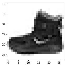
It’s a simple image, with one object, in grayscale. There’s nothing much which can be done in terms of detecting objects or their boundaries, or making any transformations (since it’s grayscale!)

So, although Fashion MNIST is more difficult than MNIST, and can be a good drop-in replacement, it does not adequately address all the concerns raised by the researchers. However, Fashion MNIST can certainly replace the original MNIST dataset for building tutorials, lessons or demonstrations for those who are new to Machine Learning or Computer Vision.